Snowflake is a powerful platform for storing and managing vast amounts of data, but makes it very easy to run up costs if one is not employing optimal practices. In this blog, I’ll discuss pruning, the holy grail of Snowflake optimization. We’ll cover the following topics:

• What is pruning and why is it important?

• The concept of clustering and its relation with pruning

• Natural clustering in Snowflake

• Programmatically identifying the top 10 expensive queries don’t use pruning

• Optimization

What is pruning, and why is it important?

Imagine you’re in a huge library with thousands of books. You’re looking for books on gardening, but this library doesn’t follow any specific order — gardening books are mixed with cookbooks, novels, and science journals. You’d have to look through each book to find what you need, which is time-consuming and exhausting.

Now, imagine if you had an awesome librarian who sorted these books into sections and labeled them. The gardening section would be in one area, all neatly organized. In this case, you’d just skip the entire cookbook and novel sections completely. Whoa, that’s a time saver!

This is pruning — saving time by skipping irrelevant sections to find out the information we seek. Snowflake, in this regard, works similar to a library — with tables instead of books. And always remember, in the Snowflake world, time = money.

Clustering and its relation with pruning

Snowflake acts like a librarian, helping to keep data organized, though it requires guidance to achieve near-human levels of intelligence. This process is known as clustering, where we define keys based on our understanding of the data and its usage. For example, in our librarian analogy, the genre of a book would be the clustering key, allowing us to quickly find what we need by skipping irrelevant sections.

Now, let’s apply this concept to a real-world scenario. In many companies, a major source of data is event data. We’ll use this as our case study to understand clustering better.

Note: While event data typically comes in JSON format, we’ll consider an example of relational data for simplicity, and to stay focused on our current topic.

Let’s consider a simple table to hold our event data.

CREATE TABLE events_data (
    event_id INTEGER,
    event_name STRING,
    event_date DATE,
    ... other event details
)

Natural clustering in Snowflake

Our event data arrives daily from a source. Snowflake intelligently recognizes this pattern and organizes the data by date automatically, a process we refer to as natural clustering. This means Snowflake can efficiently cluster data by date without any explicit instructions from us. We’ll explore another feature, Automatic Clustering, in more detail in a future blog post.

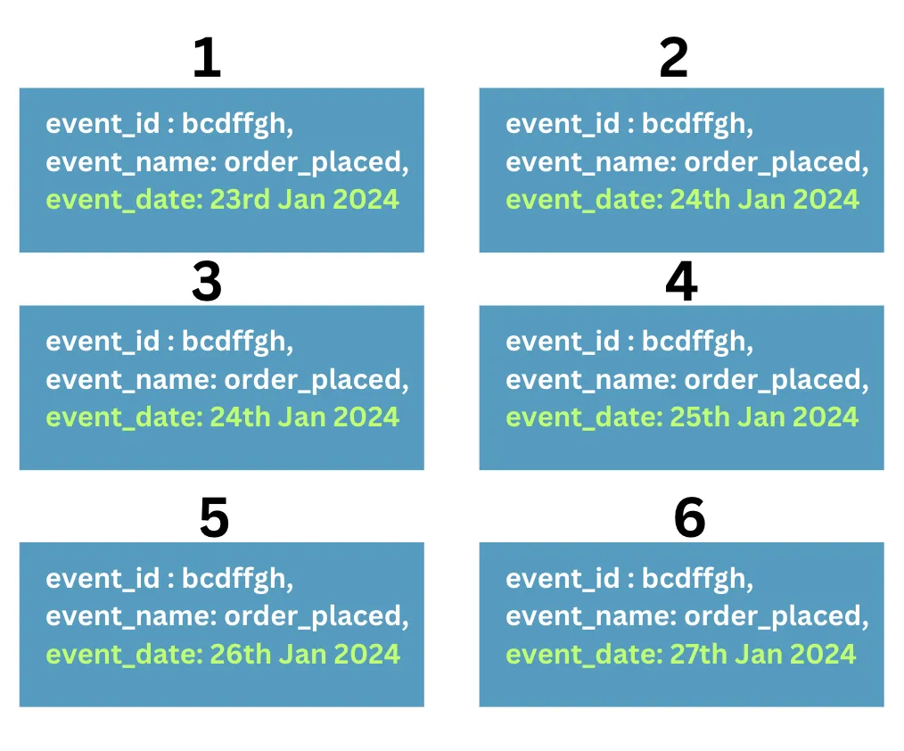
The diagram below shows how Snowflake stores event data in segments called micro-partitions. The key point is how Snowflake uses the dates of events to naturally cluster the data by event_date. When you request data for just the last three days, Snowflake cleverly filters out irrelevant micro-partitions, providing only those with event dates within this timeframe.

Finding data quickly relies on two key factors: first, organizing the data effectively, and second, understanding your requirements clearly. Just as asking a librarian for an ‘interesting’ book isn’t specific enough to save time, similarly, when retrieving data with a SQL query, it makes sense to apply a filter on the event_date column.

Identifying expensive queries that don’t use pruning

(Note: This section requires admin access for Snowflake, and will be useful if you’re looking to optimize Snowflake spend for your entire organization.)

We’ve understood pruning and clustering, but let’s delve deeper to pinpoint expensive queries that don’t utilize pruning. Our focus will be on the top 500 expensive queries over the past 14 days. We will then analyze the query plans of these queries, to identify if there are any opportunities for taking advantage of pruning.

But analyzing the query plans of 500 queries individually through the UI would be cumbersome. So we will adopt a programmatic method to identify the most important queries for review. Examining this smaller number of query plans in Snowflake’s UI would be more manageable.

Note: We lack programmatic access to queries executed more than 14 days ago.

Our strategy will be as follows:

• Identify the most expensive queries by calculating their total execution time, considering how frequently they run.

• For each identified query, we’ll programmatically retrieve their query plan using GET_QUERY_OPERATOR_STATS(<query_id>).

We’ll proceed until we’ve identified the top 10 expensive queries that aren’t pruning or have reviewed our top 500 queries.

Here’s the SQL code for Step 1:

WITH WAREHOUSE_CREDITS_MAP AS (
    SELECT * FROM (
        VALUES
            ('X-Small', 'STANDARD', 1),
            ('Small', 'STANDARD', 2),
            ('Medium', 'STANDARD', 4),
            ('Large', 'STANDARD', 8),
            ('X-Large', 'STANDARD', 16),
            ('2X-Large', 'STANDARD', 32),
            ('3X-Large', 'STANDARD', 64),
            ('4X-Large', 'STANDARD', 128),
            ('5X-Large', 'STANDARD', 256),
            ('6X-Large', 'STANDARD', 512),
            ('Medium', 'SNOWPARK-OPTIMIZED', 6),
            ('Large', 'SNOWPARK-OPTIMIZED', 12),
            ('X-Large', 'SNOWPARK-OPTIMIZED', 24),
            ('2X-Large', 'SNOWPARK-OPTIMIZED', 48),
            ('3X-Large', 'SNOWPARK-OPTIMIZED', 96),
            ('4X-Large', 'SNOWPARK-OPTIMIZED', 192),
            ('5X-Large', 'SNOWPARK-OPTIMIZED', 384),
            ('6X-Large', 'SNOWPARK-OPTIMIZED', 768)
    ) AS t (WAREHOUSE_SIZE, WAREHOUSE_TYPE, CREDITS_PER_HOUR)
),
JOINED_WITH_QUERY_HISTORY AS (
    SELECT
    qh.QUERY_TEXT, 
    qh.QUERY_ID,
    qh.EXECUTION_STATUS, 
    qh.WAREHOUSE_SIZE,
    qh.WAREHOUSE_TYPE, 
    qh.EXECUTION_TIME,
    qh.EXECUTION_TIME * wcm.CREDITS_PER_HOUR AS EFFECTIVE_EXECUTION_TIME,
    qh.USER_NAME
FROM
    SNOWFLAKE.ACCOUNT_USAGE.QUERY_HISTORY qh
JOIN
    WAREHOUSE_CREDITS_MAP wcm
ON
    wcm.WAREHOUSE_SIZE = qh.WAREHOUSE_SIZE
    AND wcm.WAREHOUSE_TYPE = qh.WAREHOUSE_TYPE
WHERE
    qh.EXECUTION_STATUS = 'FAIL'
    AND qh.START_TIME BETWEEN DATEADD('day', -14, CURRENT_DATE()) AND CURRENT_DATE()
ORDER BY EFFECTIVE_EXECUTION_TIME DESC
)
-- Step 2: Multiply the credits based on the warehouse_size to calculate
-- the effective execution time.
SELECT
    jwqh.QUERY_TEXT as QUERY_TEXT,
    MAX(jwqh.QUERY_ID) as LATEST_QUERY_ID, 
    ANY_VALUE(jwqh.WAREHOUSE_SIZE) as WAREHOUSE_SIZE,
    ANY_VALUE(jwqh.WAREHOUSE_TYPE) as WAREHOUSE_TYPE,
    AVG(jwqh.EFFECTIVE_EXECUTION_TIME::INT / 1000)::INT as AVG_EXECUTION_TIME_IN_SECONDS,
    ANY_VALUE(jwqh.USER_NAME) as USER_NAME
FROM
    JOINED_WITH_QUERY_HISTORY jwqh
    GROUP BY jwqh.QUERY_TEXT
    ORDER BY AVG_EXECUTION_TIME_IN_SECONDS DESC

Here are the sample results:

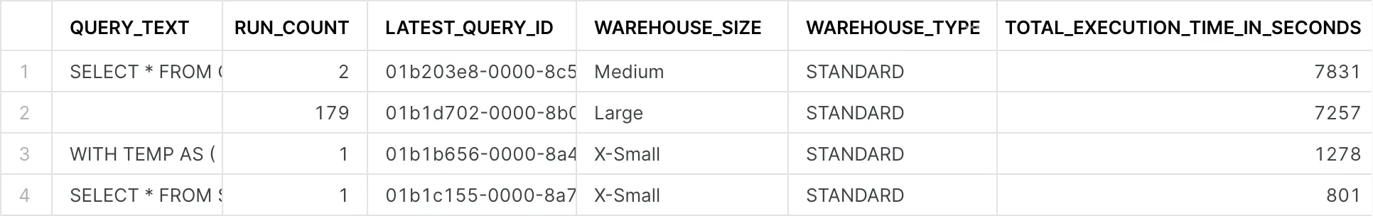
This step has helped us find out expensive queries by calculating their total execution time, while also considering the pricing of differently-sized warehouses.

Step 2: Next, we’ll identify the expensive queries that fail to effectively prune. Since there’s no direct method to access pruning details, we’ll resort to a Python script, to get a clearer structural understanding.

Our goal is to pinpoint the specific TABLE SCAN operation within a query that accounts for over 90% of its total execution time, thus identifying the culprit table. We’ll focus on analyzing the top 500 most expensive queries by cost to gather our insights. If none of these queries are returning rows, it suggests that our organization’s queries are generally well-optimized.

Why the 90% filter? To align with our goal of reducing costs, we’re targeting queries that offer the best opportunities for optimization. The first filter checks if a TABLE SCAN accounts for more than 90% of a query’s total time. The second filter examines whether 9 out of 10 partitions for the table in question are being scanned. If a query doesn’t meet these criteria, it’s not considered worth optimizing. This approach increases our chances of identifying queries where optimizations can have a significant impact.

Below is a brief code snippet for Step 2. The full, detailed code is available at the end of the article, ready to use in a Snowflake Python worksheet.

def process_query(session, query_id):
    # SQL query to extract the query operator stats for a particular query. We'll extract only the Table Scans.
    sql_query_operator_stats = f"select * from table(get_query_operator_stats('{query_id}')) where operator_type = 'TableScan'"
    df_operator_stats = session.sql(sql_query_operator_stats)
    if(df_operator_stats.count() != 0):
        query_important_stats = identify_expensive_table_scan(df_operator_stats)
        return query_important_stats
    return None

Show me the money

We now have a list of queries that are ripe for optimization. Unfortunately, there is no way to automate that actual optimization, so we’ll have to get our hands dirty. We have the relevant query IDs and the table names for each query. To extract the query texts, run the following SQL.

Select QUERY_TEXT from SNOWFLAKE.ACCOUNT_USAGE.QUERY_HISTORY 
WHERE

Let’s also run this using the table name that we have found.

SELECT SYSTEM$CLUSTERING_INFORMATION(<table_name>)

This SQL query would give us the clustering information of a particular table. If it returns an error, it implies that no explicit clustering key has been set. Note that there could still be a natural clustering key, as discussed in an earlier section.Having identifies the table names, we’ve identified which part of the query needs our attention. By examining the clustering information, we now understand which fields can be leveraged for pruning.

Now, the next step is to refine the query to fetch only the relevant data. If the clustering key is present, use that in the WHERE clause to filter out the data. If a clustering key isn’t available, we can rely on our knowledge of data insertion to use the natural clustering key for filtering. In practice, queries involving JOINS and complex predicates are often major culprits. Despite Snowflake’s innate data pruning capabilities, it cannot intuitively understand every aspect of the data.

Note: If you have followed to this point, and are interested in understanding the patterns of your data and the keys you could potentially use to cluster, check out SYSTEM$CLUSTERING_INFORMATION.